Event detection with Recurrent Neural Networks - Part 3

In this fifth lab of the ErSE 222 - Machine Learning in Geoscience course, we will use different types of Recurrent Neural Networks to detect events in noisy seismic recordings.

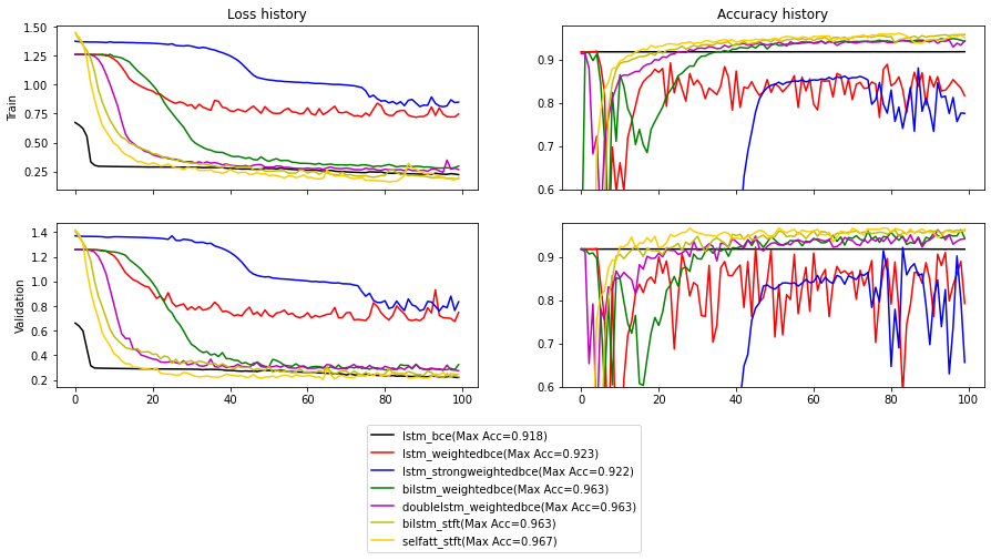
This is the final part of our lab where we compare various metrics (loss and accuracy) for the different models that we have trained.

%load_ext autoreload
%autoreload 2
%matplotlib inline

import io
import os
import glob
import random
import numpy as np
import matplotlib.pyplot as plt

modelsdir = './'

models = ['lstm_bce', 'lstm_weightedbce', 'lstm_strongweightedbce', 
          'bilstm_weightedbce', 'doublelstm_weightedbce', 
          'bilstm_stft', 'selfatt_stft']
colors = ['k', 'r', 'b', 'g', 'm', 'y', '#ffcc00']

fig, axs = plt.subplots(2, 2, sharex=True, figsize=(15, 6)) 
axs[0][0].set_title('Loss history')
axs[0][1].set_title('Accuracy history')
axs[0][0].set_ylabel('Train')
axs[1][0].set_ylabel('Validation')

for col, model in zip(colors, models):
    fhist = np.load(os.path.join(modelsdir, 'models', model + '_trainhistory.npz'))
    train_loss_history = fhist['train_loss_history']
    valid_loss_history = fhist['valid_loss_history']
    train_acc_history = fhist['train_acc_history']
    valid_acc_history = fhist['valid_acc_history']

    axs[0][0].plot(train_loss_history, col, label=model)
    axs[1][0].plot(valid_loss_history, col, label=model)
    
    axs[0][1].plot(train_acc_history, col, label=model)
    axs[1][1].plot(valid_acc_history, col, label=model + '(Max Acc=%.3f)' % valid_acc_history.max())
axs[0][1].set_ylim(0.6, 0.98)
axs[1][1].set_ylim(0.6, 0.98)

axs[1][1].legend(bbox_to_anchor=(-0.3, -0.7, 0.5, 0.5))
axs[1][1].legend(bbox_to_anchor=(-0.3, -0.7, 0.5, 0.5));

Eikonal PINN

Eikonal solver with Physics-Informed Neural Networks (PINNs) - Velocity gradient

Event Detection

Event detection with Recurrent Neural Networks - Part 3