Learning a function with PyTorch

In this third lab of the ErSE 222 - Machine Learning in Geoscience course, we will teach a neural network to learn a function, e.g. $f(x)=sin(x)$ .

Based on the Universal Approximation Theorem, we know that a NN with one hidden layer can approximate any function. We however do not know how deep it should be and how good it is at generalization. We will see that even by making the network deep, we can quite accurately interpolate our function between points but we will do poorly when we try to extrapolate outside of the domain of the training data. This is a recurring theme in ML, and especially DL, so it is worth being aware of it and what better way than considering a numerical example.

Given enough pairs $(x,f(x))$ we wish the network to be able to give us a correct estimate of $f(x_i)$ on an unseen $x_i$ .

Nevertheless, producing point estimates by means of a ML estimator does not provide us with any knowledge of how certain that estimate is. We need something that can help us understand where the model is struggling to predict (i.e., in the extrapolation regime). A variety of techniques have been development in the field of uncertainty quantification (UQ) for ML (and DL) to attach uncertainties to our estimates. See for example https://www.inovex.de/de/blog/uncertainty-quantification-deep-learning/ for a comprehesive description of some of these techniques. In this tutorial we will implement 3 of such techniques, namely:

UQ by MC-Dropout;
UQ by Distributional parameter estimation;
UQ by Deep Ensembles;
UQ by Bayesian Neural Networks.

In one of the subsequent labs we will further extend the second method for non-gaussian probabilities using Mixture Density Networks (MDNs).

%load_ext autoreload
%autoreload 2
%matplotlib inline

import random
import numpy as np
import matplotlib.pyplot as plt
import torch
import torch.nn as nn
import torch.distributions as dd
import torchbnn as bnn

from mpl_toolkits.mplot3d import Axes3D
from sklearn.datasets import make_moons
from sklearn.metrics import accuracy_score
from torch.utils.data import TensorDataset, DataLoader 
from torchsummary import summary

def set_seed(seed):
    """
    Use this to set ALL the random seeds to a fixed value and take out any randomness from cuda kernels
    """
    random.seed(seed)
    np.random.seed(seed)
    torch.manual_seed(seed)
    torch.cuda.manual_seed_all(seed)

    torch.backends.cudnn.benchmark = False
    torch.backends.cudnn.enabled   = False

    return True

Create dataset¶

set_seed(5)

True

ntrain = 64*8
ntest = 1000
sigma = 0.1 # noise standard deviation

xtrain = torch.rand(ntrain) * 10 - 6.5
xtest = torch.linspace(-6.5, 9., ntest)
ε = sigma * torch.randn(xtrain.shape[0])

ytrain = torch.sin(xtrain) + ε
ytest = torch.sin(xtest)

plt.figure()
plt.plot(xtest, ytest, 'k')
plt.plot(xtrain, ytrain, '.r')
plt.plot(xtest, ytest+2.5*sigma, '--r')
plt.plot(xtest, ytest-2.5*sigma, '--r')
plt.title('Data');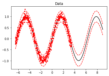

train_dataset = TensorDataset(xtrain, ytrain)
train_loader = DataLoader(train_dataset, batch_size=64, shuffle=True)

ypreds, ystds = {}, {}

Deterministic Network¶

class DeepNetwork(nn.Module):
    def __init__(self, I, H, O, drop=0.3):
        super(DeepNetwork, self).__init__()
        self.net =  nn.Sequential(
            nn.Linear(I, H[0], bias=True),
            nn.ReLU(),
            nn.Linear(H[0], H[1], bias=True),
            nn.ReLU(),
            nn.Linear(H[1], O, bias=True))
        
    def forward(self, x):
        return self.net(x)

model = DeepNetwork(1, [20, 50], 1)
model

DeepNetwork(
  (net): Sequential(
    (0): Linear(in_features=1, out_features=20, bias=True)
    (1): ReLU()
    (2): Linear(in_features=20, out_features=50, bias=True)
    (3): ReLU()
    (4): Linear(in_features=50, out_features=1, bias=True)
  )
)

optimizer = torch.optim.SGD(model.parameters(), lr=1e-2)
criterion = torch.nn.MSELoss()
n_epochs = 5000

model.train()
loss_hist = []
for epoch in range(n_epochs):
    total_loss = 0.
    for X, y in train_loader:
        optimizer.zero_grad()
        yest = model(X.view(X.shape[0], 1)).squeeze()
        loss = criterion(yest, y)
        loss.backward()
        optimizer.step()
        total_loss += loss.item()
    loss_hist.append(total_loss)
    if epoch % (n_epochs//10) == 0:
        print(f'''Epoch: {epoch}, Loss: {total_loss / X.size(0)}''')
        
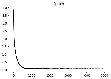
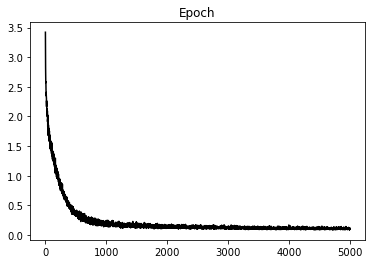
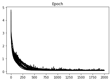
plt.figure()
plt.plot(loss_hist, 'k')
plt.title('Epoch');

Epoch: 0, Loss: 0.06033275090157986
Epoch: 500, Loss: 0.002540991597925313
Epoch: 1000, Loss: 0.001233811562997289
Epoch: 1500, Loss: 0.0012230765423737466
Epoch: 2000, Loss: 0.0011246114372625016
Epoch: 2500, Loss: 0.0011074323338107206
Epoch: 3000, Loss: 0.001136816237703897
Epoch: 3500, Loss: 0.0011185266266693361
Epoch: 4000, Loss: 0.0011437919893069193
Epoch: 4500, Loss: 0.0011770312921726145

# Prediction
ypred = model(xtest.view(xtest.shape[0], 1)) 
ypreds['Deterministic'] = ypred

plt.figure()
plt.plot(xtest, ytest, 'k')
plt.plot(xtest, ypred.detach().numpy(), '--r');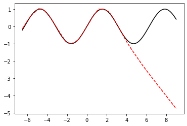

Network with Dropout UQ¶

class DeepDropNetwork(nn.Module):
    def __init__(self, I, H, O, drop=0.3):
        super(DeepDropNetwork, self).__init__()
        self.net =  nn.Sequential(
            nn.Linear(I, H[0], bias=True),
            nn.Dropout(p=drop),
            nn.ReLU(),
            nn.Linear(H[0], H[1], bias=True),
            nn.Dropout(p=drop),
            nn.ReLU(),
            nn.Linear(H[1], O, bias=True))
        
    def forward(self, x):
        return self.net(x)

model = DeepDropNetwork(1, [20, 50], 1, drop=0.01)
model

DeepDropNetwork(
  (net): Sequential(
    (0): Linear(in_features=1, out_features=20, bias=True)
    (1): Dropout(p=0.01, inplace=False)
    (2): ReLU()
    (3): Linear(in_features=20, out_features=50, bias=True)
    (4): Dropout(p=0.01, inplace=False)
    (5): ReLU()
    (6): Linear(in_features=50, out_features=1, bias=True)
  )
)

optimizer = torch.optim.SGD(model.parameters(), lr=1e-2)
criterion = torch.nn.MSELoss()
n_epochs = 5000

model.train()
loss_hist = []
for epoch in range(n_epochs):
    total_loss = 0.
    for X, y in train_loader:
        optimizer.zero_grad()
        yest = model(X.view(X.shape[0], 1)).squeeze() 
        loss = criterion(yest, y)
        loss.backward()
        optimizer.step()
        total_loss += loss.item()
    loss_hist.append(total_loss)
    if epoch % (n_epochs//10) == 0:
        print(f'''Epoch: {epoch}, Loss: {total_loss / X.size(0)}''')

plt.figure()
plt.plot(loss_hist, 'k')
plt.title('Epoch');

Epoch: 0, Loss: 0.053438459523022175
Epoch: 500, Loss: 0.005904383084271103
Epoch: 1000, Loss: 0.0023866397968959063
Epoch: 1500, Loss: 0.002072757139103487
Epoch: 2000, Loss: 0.001972118130652234
Epoch: 2500, Loss: 0.0018548647203715518
Epoch: 3000, Loss: 0.0021525937772821635
Epoch: 3500, Loss: 0.0019900686165783554
Epoch: 4000, Loss: 0.0018605671357363462
Epoch: 4500, Loss: 0.0020283856138121337

nreals = 400
yreals = np.hstack([model(xtest.view(xtest.shape[0], 1)).detach().numpy() for _ in range(nreals)])

ypred = yreals.mean(axis=1)
ystd = yreals.std(axis=1)
ypreds['Dropout'] = ypred
ystds['Dropout'] = ystd

fig, axs = plt.subplots(1, 2, sharey=True, figsize=(10, 4))
axs[0].plot(xtest, yreals, '.c', alpha=0.4)
axs[0].plot(xtest, ypred, '--b')
axs[0].plot(xtest, ytest, 'k')
axs[0].set_title('Realizations')
axs[1].plot(xtest, ytest, 'k')
axs[1].plot(xtest, ytest+2.5*sigma, '--r')
axs[1].plot(xtest, ytest-2.5*sigma, '--r')
axs[1].plot(xtest, ypred, 'b')
axs[1].fill_between(xtest, ypred - 2.5*ystd, ypred + 2.5*ystd,
                    alpha=0.5, color='b')
axs[1].set_title('Statistics')
fig.tight_layout();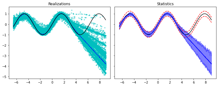

Network with Distributional parameter UQ¶

model = DeepNetwork(1, [20, 50], 2)
model

DeepNetwork(
  (net): Sequential(
    (0): Linear(in_features=1, out_features=20, bias=True)
    (1): ReLU()
    (2): Linear(in_features=20, out_features=50, bias=True)
    (3): ReLU()
    (4): Linear(in_features=50, out_features=2, bias=True)
  )
)

optimizer = torch.optim.SGD(model.parameters(), lr=1e-3)
n_epochs = 5000

model.train()
loss_hist = []
for epoch in range(n_epochs):
    total_loss = 0.
    for X, y in train_loader:
        optimizer.zero_grad()
        yest = model(X.view(X.shape[0], 1)) 
        yestdistr = dd.Normal(yest[:, 0], torch.exp(yest[:, 1]))
        loss = -torch.mean(yestdistr.log_prob(y))
        loss.backward()
        optimizer.step()
        total_loss += loss.item()
    loss_hist.append(total_loss)
    if epoch % (n_epochs//10) == 0:
        print(f'''Epoch: {epoch}, Loss: {total_loss / X.size(0)}''')

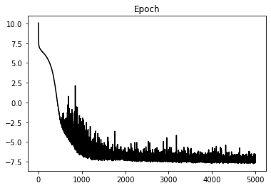
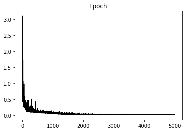
plt.figure()
plt.plot(loss_hist, 'k')
plt.title('Epoch');

Epoch: 0, Loss: 0.1573436763137579
Epoch: 500, Loss: -0.02967595378868282
Epoch: 1000, Loss: -0.08636288624256849
Epoch: 1500, Loss: -0.10893704276531935
Epoch: 2000, Loss: -0.11273339204490185
Epoch: 2500, Loss: -0.10959562007337809
Epoch: 3000, Loss: -0.09271630458533764
Epoch: 3500, Loss: -0.11049120407551527
Epoch: 4000, Loss: -0.10189047176390886
Epoch: 4500, Loss: -0.10882386472076178

nreals = 400
yest = model(xtest.view(xtest.shape[0], 1))
mu, sig = yest[:, 0], torch.exp(yest[:, 1])
ydistr = dd.Normal(mu, sig)
yreals = ydistr.sample((nreals,)).T

ypred = yreals.mean(axis=1)
ystd = yreals.std(axis=1)
ypreds['DistrPar'] = ypred
ystds['DistrPar'] = ystd

fig, axs = plt.subplots(1, 2, sharey=True, figsize=(10, 4))
axs[0].plot(xtest, yreals, '.c', alpha=0.4)
axs[0].plot(xtest, ypred, '--b')
axs[0].plot(xtest, ytest, 'k')
axs[0].set_title('Realizations')
axs[1].plot(xtest, ytest, 'k')
axs[1].plot(xtest, ytest+2.5*sigma, '--r')
axs[1].plot(xtest, ytest-2.5*sigma, '--r')
axs[1].plot(xtest, ypred, 'b')
axs[1].fill_between(xtest, ypred - 2.5*ystd, ypred + 2.5*ystd,
                    alpha=0.5, color='b')
axs[1].set_title('Statistics')
fig.tight_layout();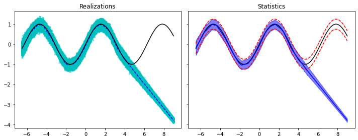

Deep Ensemble Network UQ¶

criterion = torch.nn.MSELoss()
n_epochs = 2000
n_models = 10

models = []
loss_hists = []
for i in range(n_models):
    print(f'Training model {i}/{n_models}')
    model = DeepNetwork(1, [20, 50], 1)
    optimizer = torch.optim.SGD(model.parameters(), lr=1e-2)

    model.train()
    loss_hist = []
    for epoch in range(n_epochs):
        total_loss = 0.
        for X, y in train_loader:
            optimizer.zero_grad()
            yest = model(X.view(X.shape[0], 1)).squeeze()
            loss = criterion(yest, y)
            loss.backward()
            optimizer.step()
            total_loss += loss.item()
        loss_hist.append(total_loss)
        if epoch % (n_epochs//10) == 0:
            print(f'Epoch: {epoch}, Loss: {total_loss / X.size(0)}')
    loss_hists.append(loss_hist)
    models.append(model)
    
plt.figure()
plt.plot(np.array(loss_hists).T, 'k')
plt.title('Epoch');

Training model 0/10
Epoch: 0, Loss: 0.056441571563482285
Epoch: 200, Loss: 0.013227329589426517
Epoch: 400, Loss: 0.006249168538488448
Epoch: 600, Loss: 0.003216569632058963
Epoch: 800, Loss: 0.0020202498126309365
Epoch: 1000, Loss: 0.0016170852759387344
Epoch: 1200, Loss: 0.0012992800620850176
Epoch: 1400, Loss: 0.001295278882025741
Epoch: 1600, Loss: 0.0014155734097585082
Epoch: 1800, Loss: 0.001561226454214193
Training model 1/10
Epoch: 0, Loss: 0.04955064691603184
Epoch: 200, Loss: 0.009868560009635985
Epoch: 400, Loss: 0.0023472459870390594
Epoch: 600, Loss: 0.0013725922617595643
Epoch: 800, Loss: 0.0012138907186454162
Epoch: 1000, Loss: 0.0012118900049244985
Epoch: 1200, Loss: 0.0011830247822217643
Epoch: 1400, Loss: 0.0011951664564548992
Epoch: 1600, Loss: 0.001249042667041067
Epoch: 1800, Loss: 0.0011374029345461167
Training model 2/10
Epoch: 0, Loss: 0.05348010500892997
Epoch: 200, Loss: 0.00820277800085023
Epoch: 400, Loss: 0.0022984301613178104
Epoch: 600, Loss: 0.0012926618655910715
Epoch: 800, Loss: 0.001215811149450019
Epoch: 1000, Loss: 0.0011970105915679596
Epoch: 1200, Loss: 0.0012079636435373686
Epoch: 1400, Loss: 0.0012547453152365051
Epoch: 1600, Loss: 0.0011592006485443562
Epoch: 1800, Loss: 0.0011638714422588237
Training model 3/10
Epoch: 0, Loss: 0.05076249875128269
Epoch: 200, Loss: 0.012555623427033424
Epoch: 400, Loss: 0.006098172860220075
Epoch: 600, Loss: 0.0026903237885562703
Epoch: 800, Loss: 0.0016853586566867307
Epoch: 1000, Loss: 0.0013034559451625682
Epoch: 1200, Loss: 0.0014181846199790016
Epoch: 1400, Loss: 0.0013971270600450225
Epoch: 1600, Loss: 0.0012216430041007698
Epoch: 1800, Loss: 0.001178969323518686
Training model 4/10
Epoch: 0, Loss: 0.05578446853905916
Epoch: 200, Loss: 0.005371752136852592
Epoch: 400, Loss: 0.0015205790987238288
Epoch: 600, Loss: 0.0012183480284875259
Epoch: 800, Loss: 0.0011790922580985352
Epoch: 1000, Loss: 0.0011607268315856345
Epoch: 1200, Loss: 0.0011223253241041675
Epoch: 1400, Loss: 0.0011319058321532793
Epoch: 1600, Loss: 0.0011176465050084516
Epoch: 1800, Loss: 0.0011031446701963432
Training model 5/10
Epoch: 0, Loss: 0.06215167185291648
Epoch: 200, Loss: 0.007725710573140532
Epoch: 400, Loss: 0.0027227459067944437
Epoch: 600, Loss: 0.0015588489186484367
Epoch: 800, Loss: 0.0017568397161085159
Epoch: 1000, Loss: 0.0012412187134032138
Epoch: 1200, Loss: 0.0012320931346039288
Epoch: 1400, Loss: 0.0011782761721406132
Epoch: 1600, Loss: 0.0011587112239794806
Epoch: 1800, Loss: 0.0011990456987405196
Training model 6/10
Epoch: 0, Loss: 0.07271800143644214
Epoch: 200, Loss: 0.006882586516439915
Epoch: 400, Loss: 0.0021302010281942785
Epoch: 600, Loss: 0.0013152416504453868
Epoch: 800, Loss: 0.001203377265483141
Epoch: 1000, Loss: 0.0011494948048493825
Epoch: 1200, Loss: 0.0011160683425259776
Epoch: 1400, Loss: 0.0011126006866106763
Epoch: 1600, Loss: 0.0010850060134544037
Epoch: 1800, Loss: 0.0010890436606132425
Training model 7/10
Epoch: 0, Loss: 0.057116798125207424
Epoch: 200, Loss: 0.01132946868892759
Epoch: 400, Loss: 0.004745390091557056
Epoch: 600, Loss: 0.0024609443498775363
Epoch: 800, Loss: 0.0012453992530936375
Epoch: 1000, Loss: 0.0011731840495485812
Epoch: 1200, Loss: 0.001386027186526917
Epoch: 1400, Loss: 0.0012652992154471576
Epoch: 1600, Loss: 0.0013684395016753115
Epoch: 1800, Loss: 0.0019194269989384338
Training model 8/10
Epoch: 0, Loss: 0.05405586399137974
Epoch: 200, Loss: 0.0072654044488444924
Epoch: 400, Loss: 0.0018586253863759339
Epoch: 600, Loss: 0.0013199783425079659
Epoch: 800, Loss: 0.0011732213679351844
Epoch: 1000, Loss: 0.0013286193134263158
Epoch: 1200, Loss: 0.0012906741467304528
Epoch: 1400, Loss: 0.0012882125738542527
Epoch: 1600, Loss: 0.001542336685815826
Epoch: 1800, Loss: 0.0012041646259604022
Training model 9/10
Epoch: 0, Loss: 0.07496913243085146
Epoch: 200, Loss: 0.006874952930957079
Epoch: 400, Loss: 0.002305018075276166
Epoch: 600, Loss: 0.0015276521298801526
Epoch: 800, Loss: 0.0012847651669289917
Epoch: 1000, Loss: 0.0013172833423595876
Epoch: 1200, Loss: 0.0011754585430026054
Epoch: 1400, Loss: 0.0011990106868324801
Epoch: 1600, Loss: 0.0012323572882451117
Epoch: 1800, Loss: 0.0012404082299326546

# Prediction
yreals = np.hstack([model(xtest.view(xtest.shape[0], 1)).detach().numpy() for model in models])

ypred = yreals.mean(axis=1)
ystd = yreals.std(axis=1)
ypreds['Ensemble'] = ypred
ystds['Ensemble'] = ystd

fig, axs = plt.subplots(1, 2, sharey=True, figsize=(10, 4))
axs[0].plot(xtest, yreals, '.c', alpha=0.4)
axs[0].plot(xtest, ypred, '--b')
axs[0].plot(xtest, ytest, 'k')
axs[0].set_title('Realizations')
axs[1].plot(xtest, ytest, 'k')
axs[1].plot(xtest, ytest+2.5*sigma, '--r')
axs[1].plot(xtest, ytest-2.5*sigma, '--r')
axs[1].plot(xtest, ypred, 'b')
axs[1].fill_between(xtest, ypred - 2.5*ystd, ypred + 2.5*ystd,
                    alpha=0.5, color='b')
axs[1].set_title('Statistics')
fig.tight_layout();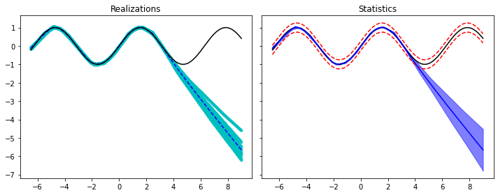

Bayesian Network¶

class BayesianNetwork(nn.Module):
    def __init__(self, I, H, O):
        super(BayesianNetwork, self).__init__()
        self.net =  nn.Sequential(
            bnn.BayesLinear(prior_mu=0, prior_sigma=0.1, in_features=I, out_features=H[0]),
            nn.ReLU(),
            bnn.BayesLinear(prior_mu=0, prior_sigma=0.1, in_features=H[0], out_features=H[1]),
            nn.ReLU(),
            bnn.BayesLinear(prior_mu=0, prior_sigma=0.1, in_features=H[1], out_features=O))
        
    def forward(self, x):
        return self.net(x)

model = BayesianNetwork(1, [20, 50], 1)
model

BayesianNetwork(
  (net): Sequential(
    (0): BayesLinear(prior_mu=0, prior_sigma=0.1, in_features=1, out_features=20, bias=True)
    (1): ReLU()
    (2): BayesLinear(prior_mu=0, prior_sigma=0.1, in_features=20, out_features=50, bias=True)
    (3): ReLU()
    (4): BayesLinear(prior_mu=0, prior_sigma=0.1, in_features=50, out_features=1, bias=True)
  )
)

optimizer = torch.optim.Adam(model.parameters(), lr=1e-2)
mse_loss = nn.MSELoss()
kl_loss = bnn.BKLLoss(reduction='mean', last_layer_only=False)
kl_weight = 0.01
n_epochs = 5000

model.train()
loss_hist = []
for epoch in range(n_epochs):
    optimizer.zero_grad()
    yest = model(xtrain.view(xtrain.shape[0], 1)).squeeze() 
    mse = mse_loss(yest, ytrain)
    kl = kl_loss(model)
    loss = mse + kl_weight*kl
    loss.backward()
    optimizer.step()
    loss_hist.append(loss.item())
    
    if epoch % (n_epochs//10) == 0:
        print(f'''Epoch: {epoch}, Loss: {loss.item()}, MSE: {mse.item()}, KL: {kl.item()}''')

plt.figure()
plt.plot(loss_hist, 'k')
plt.title('Epoch');

Epoch: 0, Loss: 0.4886898994445801, MSE: 0.47464585304260254, KL: 1.404404640197754
Epoch: 500, Loss: 0.09646101295948029, MSE: 0.07975506782531738, KL: 1.670594334602356
Epoch: 1000, Loss: 0.1044982448220253, MSE: 0.08891656249761581, KL: 1.5581680536270142
Epoch: 1500, Loss: 0.03265533968806267, MSE: 0.016974566504359245, KL: 1.5680774450302124
Epoch: 2000, Loss: 0.03826425224542618, MSE: 0.023716917261481285, KL: 1.4547337293624878
Epoch: 2500, Loss: 0.026146862655878067, MSE: 0.012891283258795738, KL: 1.3255579471588135
Epoch: 3000, Loss: 0.02823568508028984, MSE: 0.01619730331003666, KL: 1.2038382291793823
Epoch: 3500, Loss: 0.02655787393450737, MSE: 0.015229551121592522, KL: 1.1328322887420654
Epoch: 4000, Loss: 0.020889975130558014, MSE: 0.010063198395073414, KL: 1.0826776027679443
Epoch: 4500, Loss: 0.021039817482233047, MSE: 0.010568194091320038, KL: 1.0471622943878174

# Prediction
nreals = 400
yreals = np.hstack([model(xtest.view(xtest.shape[0], 1)).detach().numpy() for _ in range(nreals)])

ypred = yreals.mean(axis=1)
ystd = yreals.std(axis=1)
ypreds['BayesianNN'] = ypred
ystds['BayesianNN'] = ystd

fig, axs = plt.subplots(1, 2, sharey=True, figsize=(10, 4))
axs[0].plot(xtest, yreals, '.c', alpha=0.4)
axs[0].plot(xtest, ypred, '--b')
axs[0].plot(xtest, ytest, 'k')
axs[0].set_title('Realizations')
axs[1].plot(xtest, ytest, 'k')
axs[1].plot(xtest, ytest+2.5*sigma, '--r')
axs[1].plot(xtest, ytest-2.5*sigma, '--r')
axs[1].plot(xtest, ypred, 'b')
axs[1].fill_between(xtest.squeeze(), ypred - 2.5*ystd, ypred + 2.5*ystd,
                    alpha=0.5, color='b')
axs[1].set_title('Statistics')
fig.tight_layout();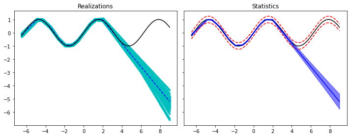

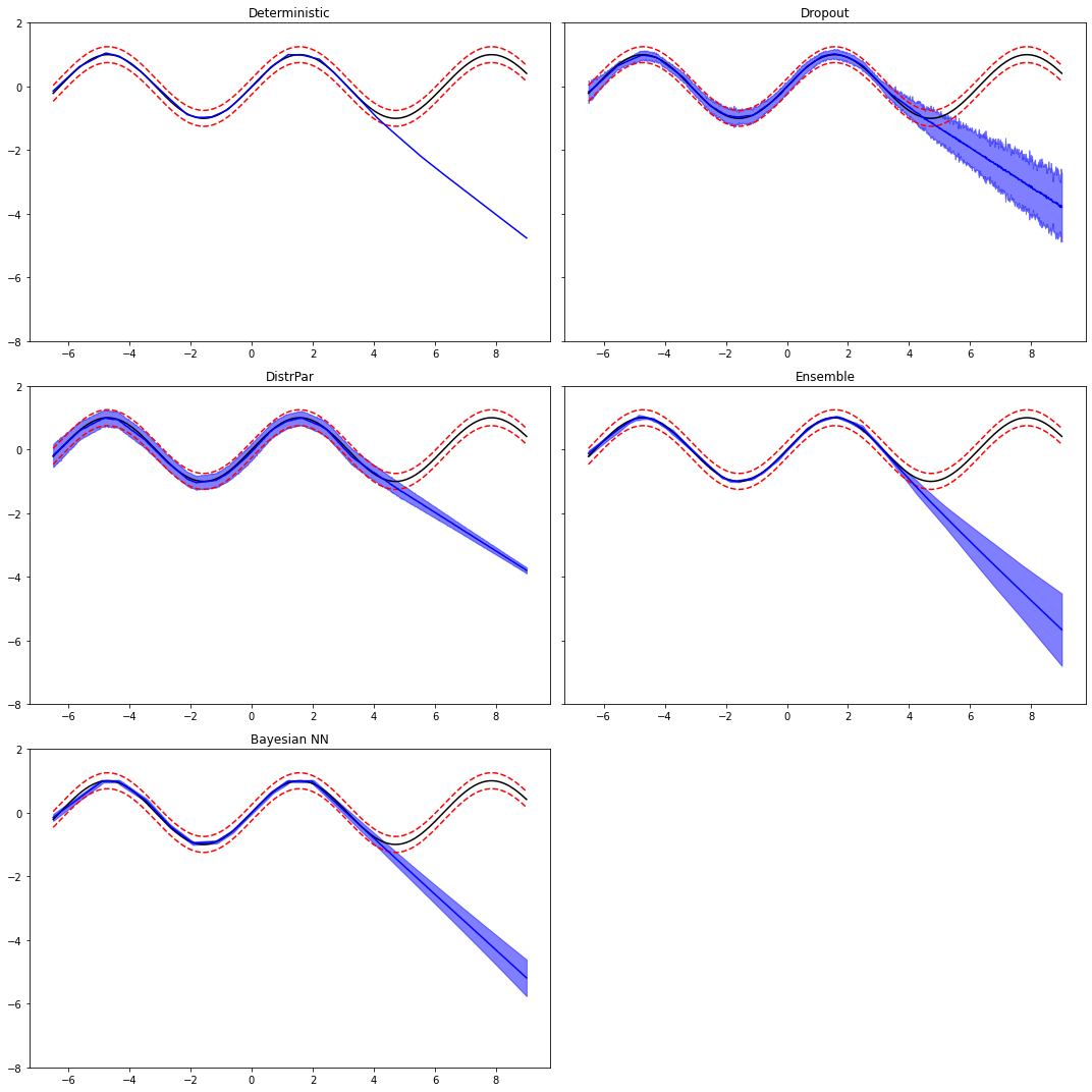
Finally, let's compare the different predictions (and their uncertainties)

fig, axs = plt.subplots(3, 2, sharey=True, figsize=(15, 15))
axs[0][0].plot(xtest, ytest, 'k')
axs[0][0].plot(xtest, ytest+2.5*sigma, '--r')
axs[0][0].plot(xtest, ytest-2.5*sigma, '--r')
axs[0][0].plot(xtest, ypreds['Deterministic'].detach().numpy(), 'b')
axs[0][0].set_title('Deterministic')
axs[0][1].plot(xtest, ytest, 'k')
axs[0][1].plot(xtest, ytest+2.5*sigma, '--r')
axs[0][1].plot(xtest, ytest-2.5*sigma, '--r')
axs[0][1].plot(xtest, ypreds['Dropout'], 'b')
axs[0][1].fill_between(xtest, ypreds['Dropout'] - 2.5*ystds['Dropout'], 
                       ypreds['Dropout'] + 2.5*ystds['Dropout'],
                       alpha=0.5, color='b')
axs[0][1].set_title('Dropout')
axs[1][0].plot(xtest, ytest, 'k')
axs[1][0].plot(xtest, ytest+2.5*sigma, '--r')
axs[1][0].plot(xtest, ytest-2.5*sigma, '--r')
axs[1][0].plot(xtest, ypreds['DistrPar'], 'b')
axs[1][0].fill_between(xtest, ypreds['DistrPar'] - 2.5*ystds['DistrPar'], 
                       ypreds['DistrPar'] + 2.5*ystds['DistrPar'],
                       alpha=0.5, color='b')
axs[1][0].set_title('DistrPar')
axs[1][1].plot(xtest, ytest, 'k')
axs[1][1].plot(xtest, ytest+2.5*sigma, '--r')
axs[1][1].plot(xtest, ytest-2.5*sigma, '--r')
axs[1][1].plot(xtest, ypreds['Ensemble'], 'b')
axs[1][1].fill_between(xtest, ypreds['Ensemble'] - 2.5*ystds['Ensemble'], 
                       ypreds['Ensemble'] + 2.5*ystds['Ensemble'],
                       alpha=0.5, color='b')
axs[1][1].set_title('Ensemble')
axs[2][0].plot(xtest, ytest, 'k')
axs[2][0].plot(xtest, ytest+2.5*sigma, '--r')
axs[2][0].plot(xtest, ytest-2.5*sigma, '--r')
axs[2][0].plot(xtest, ypreds['BayesianNN'], 'b')
axs[2][0].fill_between(xtest, ypreds['BayesianNN'] - 2.5*ystds['BayesianNN'], 
                       ypreds['BayesianNN'] + 2.5*ystds['BayesianNN'],
                       alpha=0.5, color='b')
axs[2][0].set_title('Bayesian NN')
axs[0][0].set_ylim(-8, 2)
axs[2][1].axis('off')
fig.tight_layout();

Event Detection

Event detection with Recurrent Neural Networks - Part 1

Mixture Density Network

Mixture Density Networks (MDN)