Mixture Density Networks (MDN)
In this lab of the ErSE 222 - Machine Learning in Geoscience course, we will learn about a special type of Neural Networks, called Mixture Density Networks (MDN). Their key feature is that of producing (possibly) multi-modal probabistic estimates of the network predictions parametrized as a mixture of gaussian with learned mean, standard deviation and weighting.
When compared to standard NNS, MDNs present two 3 unique elements:
A network that comprises of a:
i) backbone: takes as input and produces
ii) mixture-density layer: takes as input to 3 distinct linear layers and produces , , where is the number of gaussians in the mixture. Note that since we want to be always positive we pass this through a modified ELU activation. Similarly since we want we pass them through a softmax (here done implicitely by passing the raw outputs to a
OneHotCategoricaldistribution.A loss: negative log-likelihood (NLL). Here we first define the likelihood of the gaussian mixture
The NLL becomes:
where .
However since we are applying a logarithm to a function that involved and exponential operation this may be unstable. We therefore prefer to write an equivalent form NLL:
As you can see the formula is the same as
Evaluating the first term of the exponent is easy given . For the second term we can write its analytical expression:
A regularization (optional): MDN are hard to train due to the tendency of mode collapse. A single gaussian in the mixture is favoured and all the others are ignored. There is no ultimate solution to this problem but careful regularization can mitigate it. Two simple regularizations seem to help:
i) Weight Regularization: the L1 or L2 norms of the weights of the neurons which compute the mean, variances and mixing components are penalized.
ii) Bias Initialization: if an initial estimate of the means of the gaussians is available we can initialize the bias of the mean layers to these centers.
This notebook is organized as follows:
- A MDN is used to learn a probabilistic model from a data generated using a linear function with non-stationary noise;
- A MDN is used to learn a probabilistic model from a data generated using a gaussian mixture;
- A MDN is used to produce a probabilistic estimate of a missing well log from a suite of logs (we will use the same data as in one of our previous labs)
%load_ext autoreload
%autoreload 2
%matplotlib inline

import math
import numpy as np
import matplotlib.pyplot as plt
import torch
import torch.nn as nn
import random
import numpy as np
import pandas as pd

from scipy.stats import norm
from sklearn.metrics import mean_squared_error
from sklearn.model_selection import train_test_split
from sklearn.preprocessing import MinMaxScaler

from torch.utils.data import TensorDataset, DataLoader
from torch.distributions import Categorical
from torch.distributions import Normal, OneHotCategorical
from torch import optim
def set_seed(seed):
"""Set all random seeds to a fixed value and take out any randomness from cuda kernels
"""
random.seed(seed)
np.random.seed(seed)
torch.manual_seed(seed)
torch.cuda.manual_seed_all(seed)
torch.backends.cudnn.benchmark = False
torch.backends.cudnn.enabled = False
return Trueclass BackboneNetwork(nn.Module):
def __init__(self, in_dim, hidden_dims):
super().__init__()
# Backbone
hidden_dims = [in_dim, ] + hidden_dims
seq = []
for i in range(len(hidden_dims)-1):
seq.append(nn.Linear(hidden_dims[i], hidden_dims[i+1], bias=True))
seq.append(nn.ReLU())
self.backbone = nn.Sequential(*seq) # remove last relu
def forward(self, x):
return self.backbone(x)
class NormalNetwork(nn.Module):
def __init__(self, in_dim, out_dim, n_components):
super().__init__()
self.n_components = n_components
self.network = nn.Linear(in_dim, 2 * out_dim * n_components)
def forward(self, x):
params = self.network(x)
mean, sd = torch.split(params, params.shape[1] // 2, dim=1)
sd = nn.ELU()(sd) + 1 + 1e-15
mean = torch.stack(mean.split(mean.shape[1] // self.n_components, 1))
sd = torch.stack(sd.split(sd.shape[1] // self.n_components, 1))
return Normal(mean.transpose(0, 1), sd.transpose(0, 1)), (mean, sd)
class CategoricalNetwork(nn.Module):
def __init__(self, in_dim, out_dim):
super().__init__()
self.network = nn.Linear(in_dim, out_dim)
def forward(self, x):
params = self.network(x)
return OneHotCategorical(logits=params), params
class MixtureDensityNetwork(nn.Module):
def __init__(self, in_dim, out_dim, n_components, hidden_dims=[8, ]):
super().__init__()
self.backbone_network = BackboneNetwork(in_dim, hidden_dims)
self.pi_network = CategoricalNetwork(hidden_dims[-1], n_components)
self.normal_network = NormalNetwork(hidden_dims[-1], out_dim, n_components)
def forward(self, x):
x = self.backbone_network(x)
return self.pi_network(x), self.normal_network(x)
def loss(self, x, y):
(pi, _), (normal, _) = self.forward(x)
loglik = normal.log_prob(y.unsqueeze(1).expand_as(normal.loc))
loglik = torch.sum(loglik, dim=2)
loss = -torch.logsumexp(torch.log(pi.probs) + loglik, dim=1)
return loss
def sample(self, x):
(pi, logits), (normal, (mu, sigma)) = self.forward(x)
samples = torch.sum(pi.sample().unsqueeze(2) * normal.sample(), dim=1)
return samples, (mu, sigma, logits)def train(model, optimizer, data_loader, device='cpu'):
model.train()
loss = 0
for X, y in data_loader:
X, y = X.to(device), y.to(device)
optimizer.zero_grad()
ls = model.loss(X, y).mean()
ls.backward()
optimizer.step()
loss += ls.item()
loss /= len(data_loader)
return lossdef evaluate(model, data_loader, device='cpu'):
model.eval()
loss = 0
for X, y in data_loader:
X, y = X.to(device), y.to(device)
with torch.no_grad(): # use no_grad to avoid making the computational graph...
ls = model.loss(X, y).mean()
loss += ls.item()
loss /= len(data_loader)
return lossdef training(network, optim, nepochs, train_loader, valid_loader, device='cpu'):
iepoch_best = 0
train_loss_history = np.zeros(nepochs)
valid_loss_history = np.zeros(nepochs)
for i in range(nepochs):
train_loss = train(network, optim, train_loader, device=device)
valid_loss = evaluate(network, valid_loader, device=device)
train_loss_history[i] = train_loss
valid_loss_history[i] = valid_loss
if i % 10 == 0:
print(f'Epoch {i}, Training Loss {train_loss:.3f}, Test Loss {valid_loss:.3f}')
return train_loss_history, valid_loss_historyAs usual let's begin by checking we have access to a GPU and tell Torch we would like to use it:
device = torch.device("cuda:0" if torch.cuda.is_available() else "cpu")
print(device)
cpu
Linear function with non-stationary noise
Let's generate some synthetic data composed of a straigh line to which we add gaussian noise whose standard deviation is proportional to the square of the input.
We are using here the code in this excellent tutorial.
nsamples = 2048

# generate data
x_data = np.random.sample(nsamples)[:, np.newaxis].astype(np.float32)
y_data = np.add(5*x_data, np.multiply((x_data)**2, np.random.standard_normal(x_data.shape)))

# divide in train and validation
x_train, x_valid, y_train, y_valid = train_test_split(x_data, y_data, test_size=0.5, random_state=42)

# define test data inputs
x_test = np.linspace(0.,1.,int(1e3))[:, np.newaxis].astype(np.float32)

plt.figure(figsize=(15, 5))
plt.scatter(x_train, y_train, c='k', label='train')
plt.scatter(x_valid, y_valid, c='r', label='validation')
plt.legend();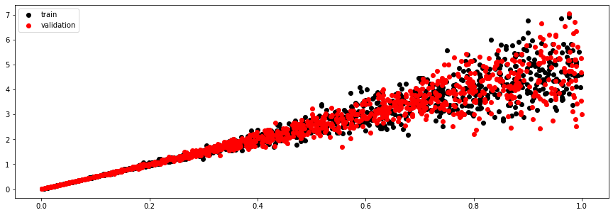
Let's start by creating a network composed of a deep backbone (2 layers with 20 and 10 hidden units) and training it with our usual training strategy
# Define Train Set
x_train = torch.Tensor(x_train)
y_train = torch.Tensor(y_train)

train_dataset = TensorDataset(x_train, y_train)

# Define Valid Set
x_valid = torch.Tensor(x_valid)
y_valid = torch.Tensor(y_valid)

valid_dataset = TensorDataset(x_valid, y_valid)

# Create DataLoaders fixing the generator for reproducibily
g = torch.Generator()
g.manual_seed(0)

train_loader = DataLoader(train_dataset, batch_size=128, shuffle=True, generator=g)
valid_loader = DataLoader(valid_dataset, batch_size=128, shuffle=False)
set_seed(5)
model = MixtureDensityNetwork(1, 1, n_components=1, hidden_dims=[20,10])
print(model)
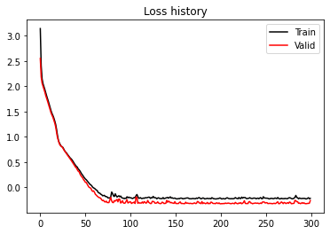
nepochs = 300
optimizer = optim.Adam(model.parameters(), lr=0.005)
train_loss_history, valid_loss_history = \
training(model, optimizer, nepochs, train_loader, valid_loader, device=device)
plt.figure()
plt.plot(train_loss_history, 'k', label='Train')
plt.plot(valid_loss_history, 'r', label='Valid')
plt.title('Loss history')
plt.legend();MixtureDensityNetwork(
(backbone_network): BackboneNetwork(
(backbone): Sequential(
(0): Linear(in_features=1, out_features=20, bias=True)
(1): ReLU()
(2): Linear(in_features=20, out_features=10, bias=True)
(3): ReLU()
)
)
(pi_network): CategoricalNetwork(
(network): Linear(in_features=10, out_features=1, bias=True)
)
(normal_network): NormalNetwork(
(network): Linear(in_features=10, out_features=2, bias=True)
)
)
Epoch 0, Training Loss 3.144, Test Loss 2.553
Epoch 10, Training Loss 1.634, Test Loss 1.584
Epoch 20, Training Loss 0.937, Test Loss 0.932
Epoch 30, Training Loss 0.655, Test Loss 0.641
Epoch 40, Training Loss 0.413, Test Loss 0.385
Epoch 50, Training Loss 0.163, Test Loss 0.098
Epoch 60, Training Loss -0.020, Test Loss -0.097
Epoch 70, Training Loss -0.164, Test Loss -0.257
Epoch 80, Training Loss -0.120, Test Loss -0.299
Epoch 90, Training Loss -0.201, Test Loss -0.297
Epoch 100, Training Loss -0.206, Test Loss -0.289
Epoch 110, Training Loss -0.213, Test Loss -0.313
Epoch 120, Training Loss -0.195, Test Loss -0.297
Epoch 130, Training Loss -0.213, Test Loss -0.288
Epoch 140, Training Loss -0.207, Test Loss -0.258
Epoch 150, Training Loss -0.223, Test Loss -0.320
Epoch 160, Training Loss -0.222, Test Loss -0.324
Epoch 170, Training Loss -0.224, Test Loss -0.313
Epoch 180, Training Loss -0.210, Test Loss -0.323
Epoch 190, Training Loss -0.205, Test Loss -0.298
Epoch 200, Training Loss -0.220, Test Loss -0.326
Epoch 210, Training Loss -0.226, Test Loss -0.319
Epoch 220, Training Loss -0.201, Test Loss -0.309
Epoch 230, Training Loss -0.218, Test Loss -0.323
Epoch 240, Training Loss -0.219, Test Loss -0.316
Epoch 250, Training Loss -0.215, Test Loss -0.308
Epoch 260, Training Loss -0.211, Test Loss -0.322
Epoch 270, Training Loss -0.226, Test Loss -0.300
Epoch 280, Training Loss -0.226, Test Loss -0.320
Epoch 290, Training Loss -0.222, Test Loss -0.303
We can now perform some predictions, first using our training data as input
y_train_pred, (mu, sigma, logits) = model.sample(x_train)

plt.figure(figsize=(15, 5))
plt.scatter(x_train, y_train, c='k', label='train')
plt.scatter(x_train, y_train_pred, c='r', label='pred')
plt.legend();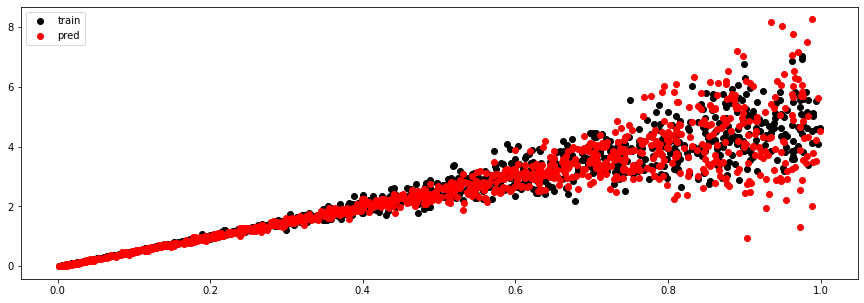
And now using the test data (which is uniformly sampled over the x axis)
x_test = torch.Tensor(x_test)
y_test, (mu, sigma, logits) = model.sample(x_test)
pi = nn.functional.softmax(logits, dim=-1)
mu_test = 5*x_test
std_test = x_test**2
plt.figure(figsize=(15, 5))
plt.scatter(x_train, y_train, c='k', label='train')
plt.scatter(x_test, y_test, c='r', label='test')
plt.legend();
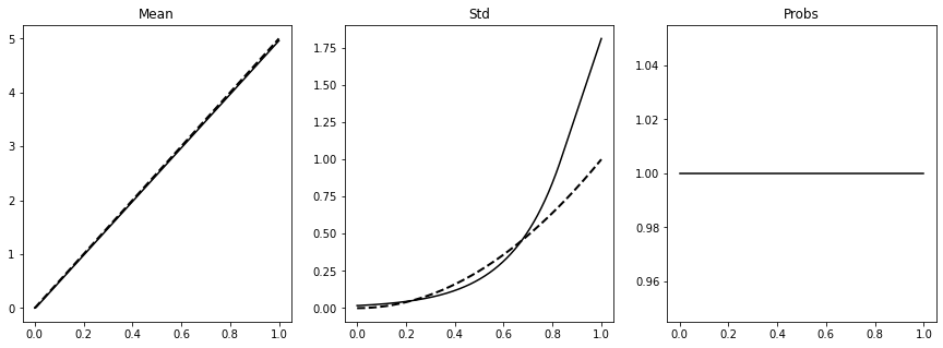
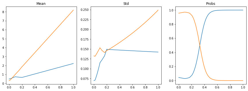
fig, axs = plt.subplots(1, 3, figsize=(15, 5))
axs[0].plot(x_test.ravel(), mu.detach().numpy().squeeze().T, 'k')
axs[0].plot(x_test.ravel(), mu_test, '--k', lw=2)
axs[0].set_title('Mean')
axs[1].plot(x_test.ravel(), sigma.detach().numpy().squeeze().T, 'k')
axs[1].plot(x_test.ravel(), std_test, '--k', lw=2)
axs[1].set_title('Std')
axs[2].plot(x_test.ravel(), pi.detach().numpy(), 'k')
axs[2].set_title('Probs');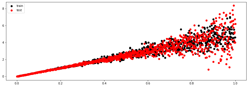
Gaussian Mixture
Let's now generate some synthetic data composed of a mixture of two gaussians
Here we slightly modify the data generation procedure from this tutorial.
nsamples = 2048

#x_data = np.random.sample(nsamples)[:, np.newaxis].astype(np.float32)
x_data = np.linspace(0,1,nsamples)[:, np.newaxis].astype(np.float32)
pi = np.sin(x_data)+3*x_data*np.cos(x_data) + 1.*np.random.sample(nsamples)[:, np.newaxis]
pi = pi/pi.max()
g1 = 2*x_data.squeeze() + 0.5*np.random.sample(nsamples)
g2 = 8*x_data.squeeze() + 0.5*np.random.sample(nsamples)

y_data = pi.round().squeeze()*g1 + (1-pi.round().squeeze())*g2
y_data = y_data.reshape(-1,1)
x_train, x_valid, y_train, y_valid = train_test_split(x_data, y_data, test_size=0.5, random_state=42)
x_test = np.linspace(0.,1.,int(1e3))[:, np.newaxis].astype(np.float32)

plt.figure(figsize=(15, 5))
plt.scatter(x_train, y_train, c='k', label='train')
plt.scatter(x_valid, y_valid, c='r', label='validation')
plt.legend();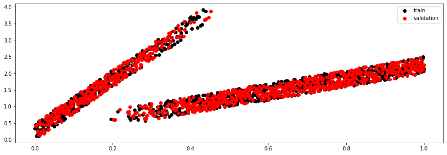
# Define Train Set
X_train = torch.from_numpy(x_train).float()
y_train = torch.from_numpy(y_train).float()

train_dataset = TensorDataset(X_train, y_train)

# Define Valid Set
X_valid = torch.from_numpy(x_valid).float()
y_valid = torch.from_numpy(y_valid).float()

valid_dataset = TensorDataset(X_valid, y_valid)

# Create DataLoaders fixing the generator for reproducibily
g = torch.Generator()
g.manual_seed(0)

train_loader = DataLoader(train_dataset, batch_size=128, shuffle=True, generator=g)
valid_loader = DataLoader(valid_dataset, batch_size=128, shuffle=False)
set_seed(5)
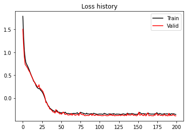
model = MixtureDensityNetwork(1, 1, n_components=2, hidden_dims=[20,10])
print(model)
nepochs = 200
optimizer = optim.Adam(model.parameters(), lr=0.005)
train_loss_history, valid_loss_history = \
training(model, optimizer, nepochs, train_loader, valid_loader, device=device)
plt.figure()
plt.plot(train_loss_history, 'k', label='Train')
plt.plot(valid_loss_history, 'r', label='Valid')
plt.title('Loss history')
plt.legend();MixtureDensityNetwork(
(backbone_network): BackboneNetwork(
(backbone): Sequential(
(0): Linear(in_features=1, out_features=20, bias=True)
(1): ReLU()
(2): Linear(in_features=20, out_features=10, bias=True)
(3): ReLU()
)
)
(pi_network): CategoricalNetwork(
(network): Linear(in_features=10, out_features=2, bias=True)
)
(normal_network): NormalNetwork(
(network): Linear(in_features=10, out_features=4, bias=True)
)
)
Epoch 0, Training Loss 1.789, Test Loss 1.506
Epoch 10, Training Loss 0.541, Test Loss 0.527
Epoch 20, Training Loss 0.212, Test Loss 0.244
Epoch 30, Training Loss -0.070, Test Loss -0.103
Epoch 40, Training Loss -0.276, Test Loss -0.304
Epoch 50, Training Loss -0.318, Test Loss -0.355
Epoch 60, Training Loss -0.342, Test Loss -0.369
Epoch 70, Training Loss -0.329, Test Loss -0.367
Epoch 80, Training Loss -0.340, Test Loss -0.384
Epoch 90, Training Loss -0.347, Test Loss -0.384
Epoch 100, Training Loss -0.350, Test Loss -0.381
Epoch 110, Training Loss -0.359, Test Loss -0.388
Epoch 120, Training Loss -0.353, Test Loss -0.385
Epoch 130, Training Loss -0.348, Test Loss -0.377
Epoch 140, Training Loss -0.348, Test Loss -0.375
Epoch 150, Training Loss -0.344, Test Loss -0.359
Epoch 160, Training Loss -0.354, Test Loss -0.388
Epoch 170, Training Loss -0.353, Test Loss -0.389
Epoch 180, Training Loss -0.350, Test Loss -0.380
Epoch 190, Training Loss -0.354, Test Loss -0.335
y_train_pred, (mu, sigma, logits) = model.sample(X_train)

plt.figure(figsize=(15, 5))
plt.scatter(X_train, y_train, c='k', label='train')
plt.scatter(X_train, y_train_pred, c='r', label='pred')
plt.legend();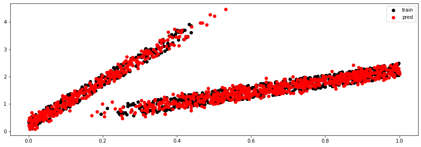
x_test = torch.Tensor(x_test)
y_test, (mu, sigma, logits) = model.sample(x_test)
pi = nn.functional.softmax(logits, dim=-1)

plt.figure(figsize=(15, 5))
plt.scatter(x_train, y_train, c='k', label='train')
plt.scatter(x_test, y_test, c='r', label='test')
plt.plot(x_test.ravel(), mu.detach().numpy().squeeze().T, 'k')
plt.legend()
plt.ylim(0,5)

fig, axs = plt.subplots(1, 3, figsize=(15, 5))
axs[0].plot(x_test.ravel(), mu.detach().numpy().squeeze().T)
axs[0].set_title('Mean')
axs[1].plot(x_test.ravel(), sigma.detach().numpy().squeeze().T)
axs[1].set_title('Std')
axs[2].plot(x_test.ravel(), pi.detach().numpy())
axs[2].set_title('Probs');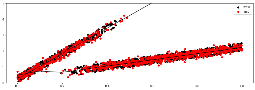
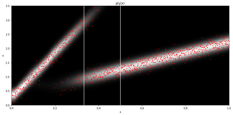
nyax = 101
yax = np.linspace(-0.5, 3.5, nyax)
Py = np.zeros((len(x_test), nyax))
for i in range(len(x_test)):
Py[i] = pi[i, 0].detach().numpy() * norm.pdf(yax, float(mu[0, i,0].detach().numpy()), float(sigma[0, i, 0].detach().numpy())) + \
pi[i, 1].detach().numpy() * norm.pdf(yax, float(mu[1, i,0].detach().numpy()), float(sigma[1, i, 0].detach().numpy()))
plt.figure(figsize=(15, 7))
plt.imshow(Py.T, cmap='gray', extent=(x_test[0][0], x_test[-1][0], 3.5, -0.5))
plt.scatter(x_test.ravel(), y_test.ravel(), c='r', s=3)
plt.axvline(x_test[len(x_test)//3], c='w')
plt.axvline(x_test[len(x_test)//2], c='w')
plt.xlabel('x')
plt.ylabel('y')
plt.title('p(y|x)')
plt.axis('tight')
plt.ylim(0, 3.5);
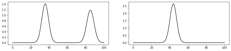
fig, axs = plt.subplots(1, 2, figsize=(15, 3))
axs[0].plot(Py[len(x_test)//3], 'k')
axs[1].plot(Py[len(x_test)//2], 'k')/Users/ravasim/opt/anaconda3/envs/mlcourse/lib/python3.8/site-packages/numpy/core/_asarray.py:102: FutureWarning: The input object of type 'Tensor' is an array-like implementing one of the corresponding protocols (`__array__`, `__array_interface__` or `__array_struct__`); but not a sequence (or 0-D). In the future, this object will be coerced as if it was first converted using `np.array(obj)`. To retain the old behaviour, you have to either modify the type 'Tensor', or assign to an empty array created with `np.empty(correct_shape, dtype=object)`.
return array(a, dtype, copy=False, order=order)
[<matplotlib.lines.Line2D at 0x7f8dfdc85370>]